Plotting the results for each statistical model from the reslr_mcmc function.

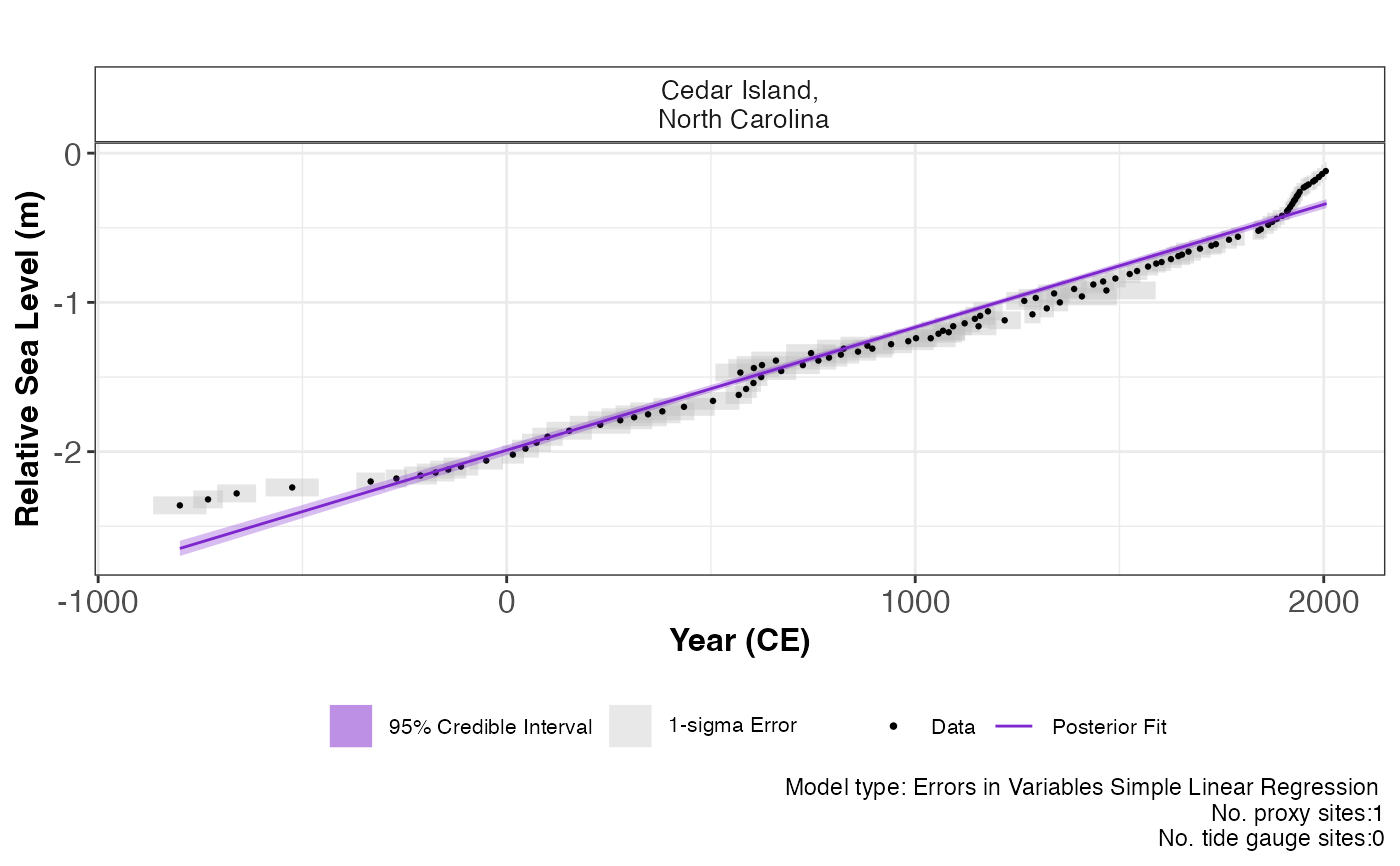
Depending on the model chosen in the reslr_mcmc function, the package produces a range of output plots. Total posterior model fit plot with the raw data and measurement uncertainty are created for each statistical model. The rate of change plots are created for the EIV IGP and the NI spline regression models. For the NI GAM decomposition, each individual component of the model is plotted. Also, the regional and the non-linear local component, an associated rate plot is produced. If tide gauges are used in the model, the user has the ability plot the output with or without this additional data source.

# S3 method for reslr_output
plot(
  x,
  plot_proxy_records = TRUE,
  plot_tide_gauges = FALSE,
  title = "",
  plot_type = c("model_fit_plot"),
  plot_caption = TRUE,
  xlab = "Year (CE)",
  ylab = "Relative Sea Level (m)",
  y_rate_lab = "Rate of change (mm per year)",
  ...
)

Arguments

x

An object of class reslr_output and model_type created via reslr_mcmc

plot_proxy_records

Plotting the proxy records on their own and this is the default

plot_tide_gauges

Plotting the tide gauge data as well as proxy data

title

Plotting a title on the output plots

plot_type

The user can select the type of output plot they require from the following: "rate_plot", "model_fit_plot", "regional_plot", "regional_rate_plot", "linear_local_plot", "non_linear_local_plot", "non_linear_local_rate_plot", "nigam_component_plot"

plot_caption

Plotting an informed caption with the number of tide gauges and proxy sites.

xlab

Labeling the x-axis

ylab

Labeling the y-axis

y_rate_lab

Labeling the y-axis for rate of change plots

...

Not used

Value

Plot of model fit and the rate of change depending on the statistical model in question.

Examples

# \donttest{
data <- NAACproxydata %>% dplyr::filter(Site == "Cedar Island")
x <- reslr_load(data = data)
jags_output <- reslr_mcmc(x, model_type = "eiv_slr_t")
#> Compiling model graph
#>    Resolving undeclared variables
#>    Allocating nodes
#> Graph information:
#>    Observed stochastic nodes: 208
#>    Unobserved stochastic nodes: 107
#>    Total graph size: 1003
#> 
#> Initializing model
#> 
plot(x = jags_output)# }